Penguins 인공신경망

Penguins, 인공신경망 구성
도입
Penguins 데이터로 인공신경망 만들기
인공신경망을 공부하는MNIST를 자주 사용하곤 하지만, MNIST의 index는 60,000개로 사이즈가 크기 때문에 학습에 시간이 오래 걸린다.
그래서 데이터 사이즈가 작고 귀여운 Penguins 데이터로 인공신경망을 연습하자
데이터 전처리
데이터 읽어오기
# Data Load
penguins = sns.load_dataset('penguins')
print(f"🎬 Rows, Columns : {penguins.shape}")
# 🎬 Rows, Columns : (344, 7)
- 데이터는 Seaborn에서 불러왔다.
- 데이터에 대한 자세한 설명은 Seaborn 링크 참조 해주세요
특성공학
- 특별한 특성공학은 하지 않음
- sex가 결측인 경우 3으로 대체
- 다른 특성은 평균으로 대체
penguins_species = {
    'Adelie' : 0,
    'Gentoo' : 1,
    'Chinstrap' : 2,
}
penguins['species'] = penguins['species'].map(penguins_species)

penguins_island = {
    'Biscoe' : 0,
    'Dream' : 1,
    'Torgersen' : 2,
}
penguins['island'] = penguins['island'].map(penguins_island)

penguins_sex = {
    'Male' : 0,
    'Female' : 1,
    np.nan : 3,
}
penguins['sex'] = penguins['sex'].map(penguins_sex)

# NaN = Fill with Mean
for idx, col in enumerate(penguins.columns):
  penguins[col].fillna(penguins[col].mean(), inplace=True)
데이터 분할
test_size = 0.2
x_train, x_test, y_train, y_test = train_test_split(penguins[features], penguins[target], test_size=test_size, random_state=rand_seed)
print(f'✨Train Shape : {x_train.shape} / {y_train.shape}\n🎉 Test Shape : {x_test.shape} / {y_test.shape}')
#✨Train Shape : (275, 6) / (275, 1)
#🎉 Test Shape : (69, 6) / (69, 1)
정규화(Normalization)
x_train = (x_train - np.min(x_train, axis='index')) / (np.max(x_train, axis='index') - np.min(x_train, axis='index'))
x_test  = ( x_test - np.min( x_test, axis='index')) / (np.max( x_test, axis='index') - np.min( x_test, axis='index'))
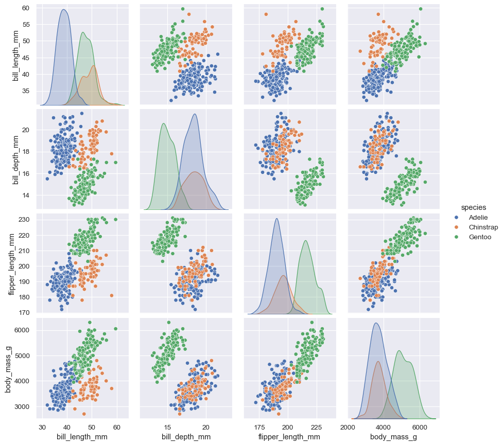
탐색적 데이터 분석
Seaborn 의 데이터 소개로 대체

모델링
기준모델 : Logistic Regression
- 로지스틱 회귀분석모델을 기준모델로 하자!
log_model = LogisticRegression()
log_model.fit(x_train, y_train)
log_score = print_accuracy(log_model)
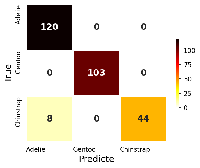
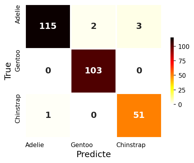
log_CM, fig = draw_CM(log_model)
# Train Accuracy : 0.978, Test Accuracy : 0.971
- 기준모델 정확도가 무려 97.1% 😳 (큰일이다…)
- 보통은 기준모델 이상을 목표로 하지만 오늘은 기준모델 만큼이라도 달성하는 것을 목표로 하자

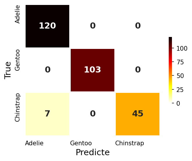
기본 인공신경망 : 은닉층 0개
- 가장 기본적인 인공신경망을 만들어보자
model1 = tf.keras.Sequential([
    Dense(3, activation='softmax'),
    ])

model1.compile(metrics=['accuracy']
               , optimizer='adam'
               , loss='sparse_categorical_crossentropy'
               )

results1 = model1.fit(x_train, y_train
                      , epochs=5
                      , verbose=0
                      )

model1_score = print_accuracy(model1)
log_CM, fig = draw_CM(model1)
model1.summary()
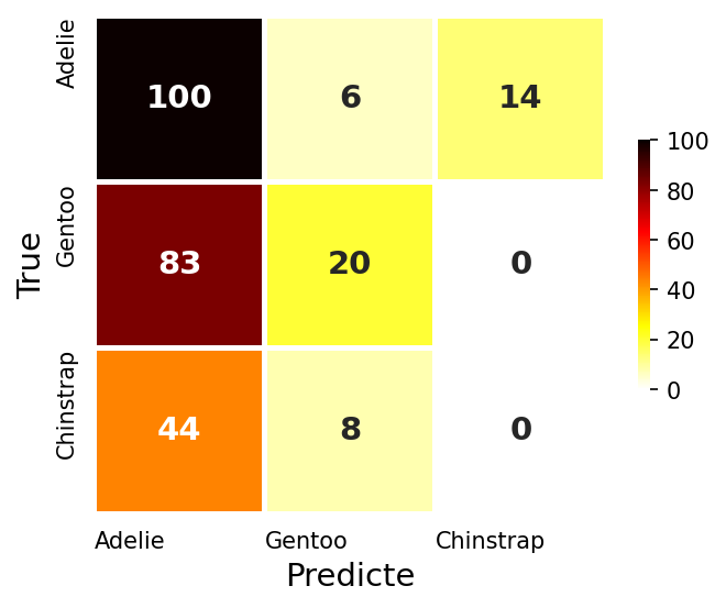
- 은닉층 없이 출력증에만 펭귄종류 3가지만 지정하고, 다중분류 활성화함수인 softmax 지정
- 최소한의 학습을 위하여 epochs를 5로 지정
- 입력 특성 7개, 출력 타겟클래스 3개, Total 파라미터 21개
- 평가 정확도 53.6%…😭😢😞 (딥러닝… 버려야 하나?)
# Train Accuracy : 0.436, Test Accuracy : 0.536
_________________________________________________________________
 Layer (type)                Output Shape              Param #
=================================================================
 dense_37 (Dense)            (None, 3)                 21

=================================================================
Total params: 21
Trainable params: 21
Non-trainable params: 0
_________________________________________________________________
기본 인공신경망 : 은닉층 1개
- 은닉층을 하나 만들어 보자
model1 = tf.keras.Sequential([
    Dense(100, activation='relu', kernel_initializer='he_uniform'),
    Dense(3, activation='softmax'),
    ])

model1.compile(metrics=['accuracy']
               , optimizer='adam'
               , loss='sparse_categorical_crossentropy'
               )

results1 = model1.fit(x_train, y_train
                      , epochs=5
                      , verbose=0
                      )

model1_score = print_accuracy(model1)
log_CM, fig = draw_CM(model1)
model1.summary()
- 하나의 은닉층에 노드 100개, 활성화함수는 ReLU, 가중치 초기화는 ‘he_uniform’을 지정
- 은닉층이 생기면서 추정해야 할 파라미터가 1,003개로 늘었다.
- 평가 정확도 76.8%!!
# Train Accuracy : 0.807, Test Accuracy : 0.768
_________________________________________________________________
 Layer (type)                Output Shape              Param #
=================================================================
 dense_38 (Dense)            (None, 100)               700

 dense_39 (Dense)            (None, 3)                 303

=================================================================
Total params: 1,003
Trainable params: 1,003
Non-trainable params: 0
기본 인공신경망 : 은닉층 2개
- 일반적으로 딥러닝이라 하면 은닉층이 2개 이상을 의미한다.
- 은닉층을 2개 추가해보자
model1 = tf.keras.Sequential([
    Dense(100, activation='relu', kernel_initializer='he_uniform'),
    Dense(100, activation='relu', kernel_initializer='he_uniform'),
    Dense(3, activation='softmax'),
    ])

model1.compile(metrics=['accuracy']
               , optimizer='adam'
               , loss='sparse_categorical_crossentropy'
               )

results1 = model1.fit(x_train, y_train
                      , epochs=5
                      , verbose=0
                      )

model1_score = print_accuracy(model1)
log_CM, fig = draw_CM(model1)
model1.summary()
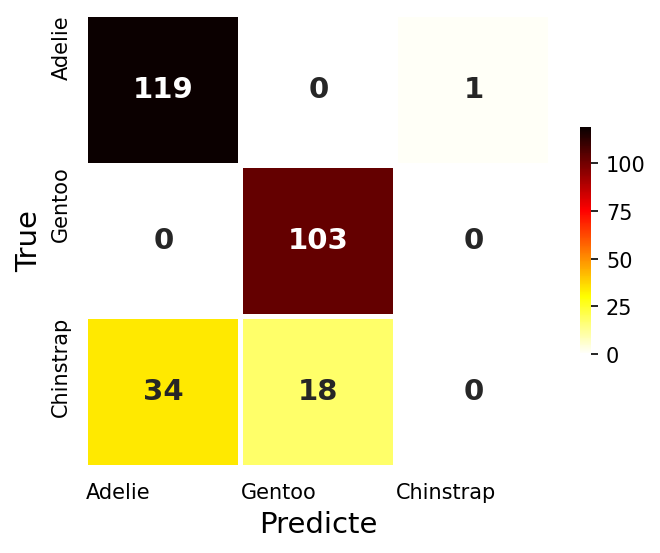
- 똑같은 은닉층을 2개로 늘렸다
- 평가 정확도 95.7%🎉
# Train Accuracy : 0.971, Test Accuracy : 0.957
_________________________________________________________________
 Layer (type)                Output Shape              Param #
=================================================================
 dense_40 (Dense)            (None, 100)               700

 dense_41 (Dense)            (None, 100)               10100

 dense_42 (Dense)            (None, 3)                 303

=================================================================
Total params: 11,103
Trainable params: 11,103
Non-trainable params: 0
- 인공신경망의 은닉층이 2개 이상으로 늘어나지깐 정확도가 급 상승했다
인공신경망 실험
실험1 : 은닉층의 수를 늘리면 성능이 오늘까?
- 은닉층 1개 ~ 99개 까지 모델을 학습하고 정확도를 비교해보자
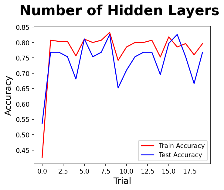
- 2개 이후로는 성능의 향상이 크게 없는 것 같다
- 앞으로는 효율성을 위하여 은닉층은 2개로 고정할 것이다
실험2 : 은닉층의 노드를 늘리면 성능이 오를까?
- 은닉층의 노드는 가중치와 편향의 가중합 연산이 일어나는 부분이다.
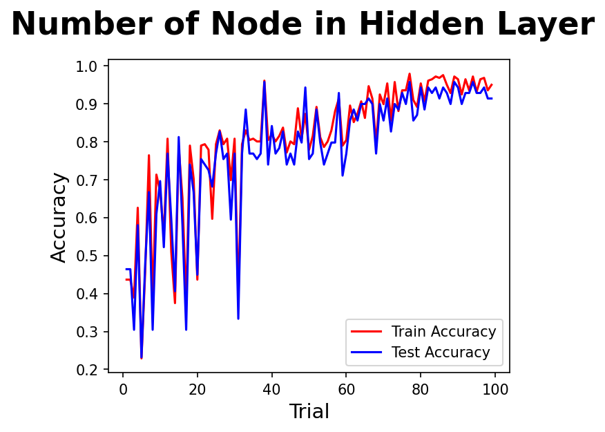
- 은닉층이 오르면서 성능도 오르고, 성능의 안정감도 오르는 것 같다.
- 노드 80 이후로는 큰 차이가 없어보인다.
- 앞으로는 노드를 100정도로 고정할 것이다
실험3 : 은닉층의 모양은 성능과 어떤 상관이 있을까?
- 2개 은닉층의 노드 비율을 1:99 , 2:98 , 3:97 …… 98:2 , 99:1 로 변화시켜 보자
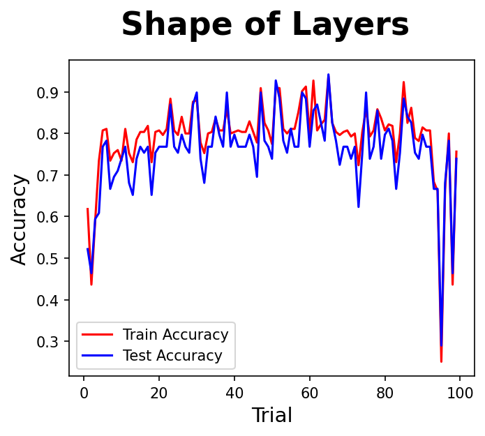
- 2개 은닉층의 비율이 크게 차이나는 1:99, 2:98 … 98:2, 99:1 은 성능 점수도 낮고, 안정감도 떨어지는 것 같다.
- 은닉층의 비율은 비슷한 것이 좋겠다.
최적 Layer 모델
- 지금까지의 실험을 토대로 딥러닝 모델을 만들어보자
def get_model(nodes=100, lr=0.001):
    random.seed(rand_seed)
    model = tf.keras.Sequential([
                                Dense(nodes, activation='relu', kernel_initializer='he_uniform'),
                                Dense(nodes, activation='relu', kernel_initializer='he_uniform'),
                                Dense(3, activation='softmax'),
                                ])

    model.compile(metrics=['accuracy']
                  , optimizer=tf.keras.optimizers.Adam(learning_rate=lr)
                  , loss='sparse_categorical_crossentropy'
                  )

    return model
- 앞으로의 실험은 아래의 모델을 중심으로 실행할 것이다
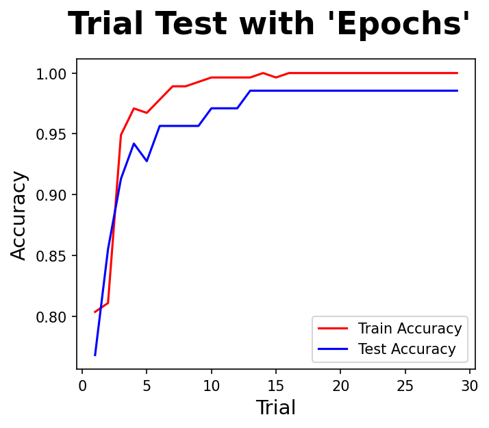
실험4 : epochs
- epoch는 인공신경망이 순전파와 역전파를 통하여 1회 학습이 일어나는 과정이다.
- 인공신경망에서는 역전파를 통하여 모델의 업데이트가 일어나기 때문에 epoch가 많아지면 모델이 정교해질 가능성이 있다.
- epoch를 1~30 까지 조정하며 정확도를 평가해보자
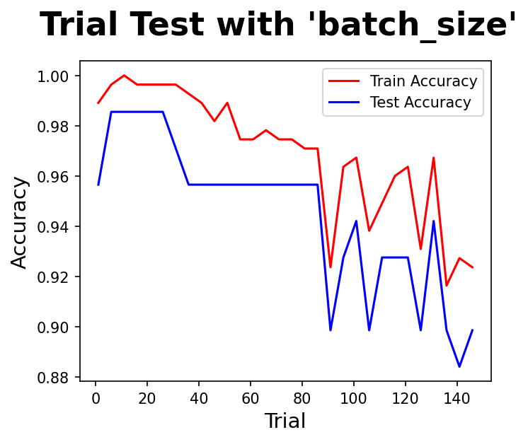
실험5 : batch_size
- 경사하강법을 통하여 손실함수를 계산할 때 전통적으로는 모든 입력데이터에 대하여 계산을 수행하였다.
- 데이터가 커지면서 시간이 오래걸리고 비효율성이 높아져 확률적 경사하강법, 곧 일부데이터를 뽑아서 손실함수를 계산하는 방법이 생겨났다.
- batch_size를 지정한면 그만큼 입력데이터를 뽑아 미니배치(Mini-batch) 경사하강법을 수행하게 된다.
- 이때 입력데이터 수, batch_size, iteration은 다음과 같은 관계가 성립된다.
- $Nobs. Data = batch_size \times Iteration(by \; epoch)$
- 실험 결과 80 이하가 적당한 것 같다.
학습률 계획
- 가장 중요한 하이퍼파라미터 가운데 하나가 바로 학습률(Learning Rate)이다.
- 인공신경망에서 가중치 업데이트는 다음과 같은 계산으로 수행된다.
- $\theta_{ i,j+1 } = \theta_{ i,j } - \eta { { \delta }\over{ \delta \theta_{ i,j } } }J(\theta)$
- $\theta_{ i,j+1 }$ : 새롭게 생신된 가중치
- $\theta_{ i,j }$ : 갱신 전 가중치
- $\eta$ : 학습률
- ${ { \delta }\over{ \delta \theta_{ i,j } } }J(\theta)$ : 해당 지점에서의 기울기
- 그래서 학습률은 가중치 업데이트과정 가운데 가중치의 변화폭이라고 이해할 수 있다.
- 학습률은 직업 지정해줄 수도 있지만 주로 Step Decay, Cosine Decay의 두가지 방식이 자주 사용된다.
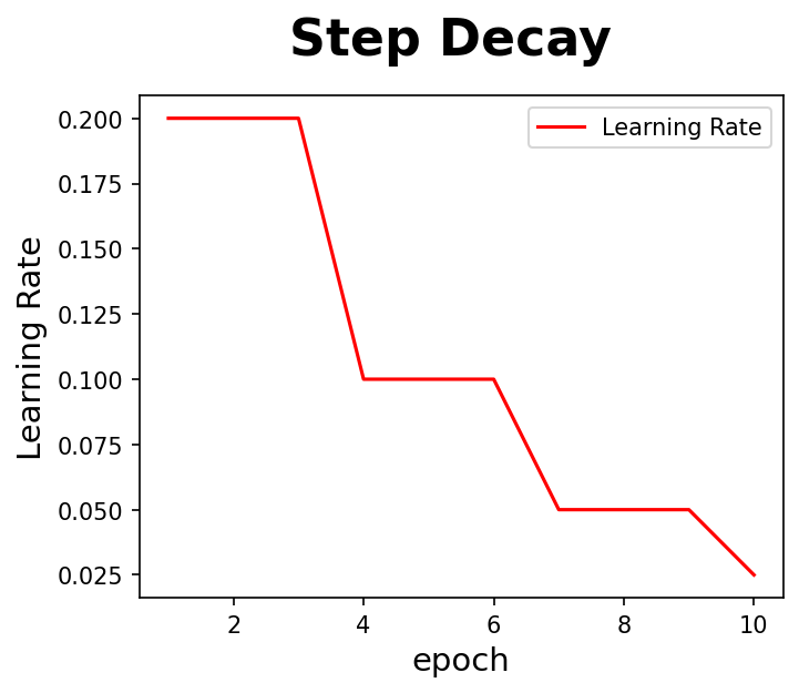
학습률 Step Decay
- 학습률 Step Decay는 사용자 함수를 만들어 LearningRateScheduler() 메써드에 담아 콜백으로 학습과정으로 넘겨주면 된다.
# 학습률 Step Decay를 위한 함수
def step_decay(epoch):
    start = 0.2
    drop = 0.5
    epochs_drop = 3
    lr = start * (drop ** np.floor((epoch)/epochs_drop))
    return lr

lr_scheduler = LearningRateScheduler(step_decay, verbose=0)

model = get_model()

model_results = model.fit(x_train, y_train
                          , batch_size              = 16 # None
                          , epochs                  = 10 # 1
                          , verbose                 = 0 # 'auto'
                          , callbacks               = [lr_scheduler] # None
                          )

model_accuracy = print_accuracy(model, verbose=1)

# 그래프 그리기
fig, ax = plt.subplots( figsize=(5, 4) )
fig.suptitle('Step Decay', fontsize = 22, fontweight = 'bold', y = 1)

sns.lineplot(x=range(1,11), y=model_results.history['lr'], color='r', label='Learning Rate')

plt.xlabel('epoch', fontsize = 14)
plt.ylabel('Learning Rate', fontsize = 14)
plt.show()
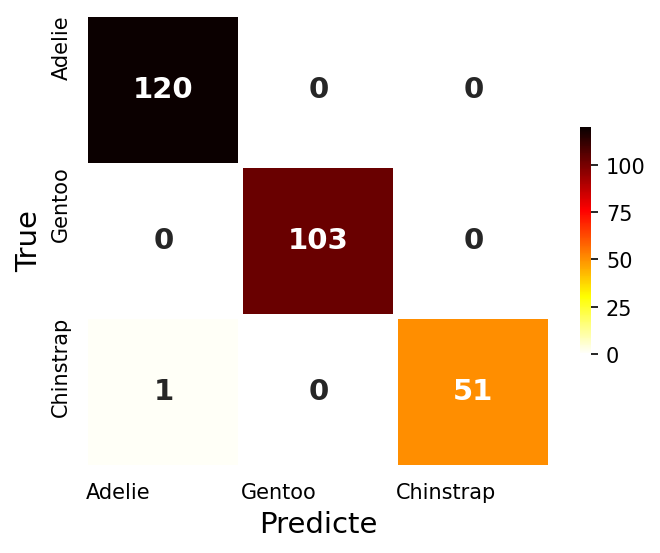
- 학습률이 epoch가 진행됨에 따라 만든 함수에 따라서 감소하는 것을 볼 수 있다.
- Train Accuracy : 0.996, Test Accuracy : 0.986
학습률 Cosine Decay
- 학습률 Cosine Decay 는 코사인의 형태로 학습률을 감소시킨다.
- Step Decay처럼 급격하게 학습률이 변하는 것이 아니라 코사인 곡선을 그리며 학습률이 미세하게 감소하도록 할 수 있다.
- Train Accuracy : 0.913, Test Accuracy : 0.971
first_decay_steps = 1000
initial_learning_rate = 0.2

# Cosine Learning Rate Decay
cos_decay = (
  tf.keras.experimental.CosineDecayRestarts(
      initial_learning_rate,
      first_decay_steps)
  )

model = get_model(lr=cos_decay)

model_results = model.fit(x_train, y_train
                          , batch_size              = 16 # None
                          , epochs                  = 10 # 1
                          , verbose                 = 0 # 'auto'
                          )

model_accuracy = print_accuracy(model, verbose=1)
과적합 방지
가중치 감소(Weight Decay)
- 가중치 감소를 위한 정규화는 L1 Regularization(LASSO), L2 Regularization(Ridge)의 두 가지가 있다.
- kernel_regularizer, activity_regularizer의 차이는 아직 모르겠다.
- Train Accuracy : 0.993, Test Accuracy : 0.957
- 점수가 잘 나오니 일단 사용하자…😳
first_decay_steps = 1000
initial_learning_rate = 0.2

# Cosine Learning Rate Decay
cos_decay = (
  tf.keras.experimental.CosineDecayRestarts(
      initial_learning_rate,
      first_decay_steps)
  )

model = tf.keras.Sequential([
                            Dense(100
                                  , activation='relu'
                                  , kernel_initializer='he_uniform'
                                  , kernel_regularizer=L1(0.01)
                                  , activity_regularizer=L2(0.01)
                                  ),
                            Dense(100
                                  , activation='relu'
                                  , kernel_initializer='he_uniform'
                                  , kernel_regularizer=L2(0.01)
                                  , activity_regularizer=L1(0.01)
                                  ),
                            Dense(3, activation='softmax'),
                            ])

model.compile(metrics=['accuracy']
              , optimizer=tf.keras.optimizers.Adam(learning_rate=0.001)
              , loss='sparse_categorical_crossentropy'
              )

model_results = model.fit(x_train, y_train
                          , batch_size              = 16 # None
                          , epochs                  = 10 # 1
                          , verbose                 = 0 # 'auto'
                          )

model_accuracy = print_accuracy(model, verbose=1)
Dropout
- 은닉층의 일부 노드를 학습에 사용하지 않도록하여 과적합을 방지하는 방법이다.
- 은닉층 뒤에 Dropout(0.5) 메써드를 추가하여 설정할 수 있다.
- Train Accuracy : 0.975, Test Accuracy : 0.957
first_decay_steps = 1000
initial_learning_rate = 0.2

# Cosine Learning Rate Decay
cos_decay = (
  tf.keras.experimental.CosineDecayRestarts(
      initial_learning_rate,
      first_decay_steps)
  )

model = tf.keras.Sequential([
                            Dense(100
                                  , activation='relu'
                                  , kernel_initializer='he_uniform'
                                  , kernel_regularizer=L1(0.01)
                                  , activity_regularizer=L2(0.01)
                                  ),
                            Dense(100
                                  , activation='relu'
                                  , kernel_initializer='he_uniform'
                                  , kernel_regularizer=L2(0.01)
                                  , activity_regularizer=L1(0.01)
                                  ),
                            Dropout(0.5),
                            Dense(3, activation='softmax'),
                            ])

model.compile(metrics=['accuracy']
              , optimizer=tf.keras.optimizers.Adam(learning_rate=0.001)
              , loss='sparse_categorical_crossentropy'
              )

model_results = model.fit(x_train, y_train
                          , batch_size              = 16 # None
                          , epochs                  = 10 # 1
                          , verbose                 = 0 # 'auto'
                          )

model_accuracy = print_accuracy(model, verbose=1)
Early Stopping
- 과정합이 심해지기 전에 학습을 멈추도록 설정
first_decay_steps = 1000
initial_learning_rate = 0.2

# Cosine Learning Rate Decay
cos_decay = (
  tf.keras.experimental.CosineDecayRestarts(
      initial_learning_rate,
      first_decay_steps)
  )

# Early Stopping
early_stop = keras.callbacks.EarlyStopping(monitor='val_accuracy', min_delta=0, patience=3, verbose=1)

model = tf.keras.Sequential([
                            Dense(100
                                  , activation='relu'
                                  , kernel_initializer='he_uniform'
                                  , kernel_regularizer=L1(0.01)
                                  , activity_regularizer=L2(0.01)
                                  ),
                            Dense(100
                                  , activation='relu'
                                  , kernel_initializer='he_uniform'
                                  , kernel_regularizer=L2(0.01)
                                  , activity_regularizer=L1(0.01)
                                  ),
                            Dropout(0.5),
                            Dense(3, activation='softmax'),
                            ])

model.compile(metrics=['accuracy']
              , optimizer=tf.keras.optimizers.Adam(learning_rate=0.001)
              , loss='sparse_categorical_crossentropy'
              )

model_results = model.fit(x_train, y_train, validation_data=(x_test, y_test)
                          , batch_size        = 16 # None
                          , epochs            = 20 # 1
                          , verbose           = 1 # 'auto'
                          , callbacks         = [early_stop]
                          )

model_accuracy = print_accuracy(model, verbose=1)
- 다음과 같이 11번째 epoch에서 과적합이 발생해 학습이 중단되었다
- Train Accuracy : 0.982, Test Accuracy : 0.957
Epoch 1/20
18/18 [==============================] - 1s 17ms/step - loss: 6.1275 - accuracy: 0.6509 - val_loss: 5.5955 - val_accuracy: 0.7681
Epoch 2/20
18/18 [==============================] - 0s 6ms/step - loss: 5.4336 - accuracy: 0.7891 - val_loss: 5.1008 - val_accuracy: 0.8551
Epoch 3/20
18/18 [==============================] - 0s 6ms/step - loss: 4.9484 - accuracy: 0.8691 - val_loss: 4.7225 - val_accuracy: 0.8551
Epoch 4/20
18/18 [==============================] - 0s 5ms/step - loss: 4.5982 - accuracy: 0.8764 - val_loss: 4.4008 - val_accuracy: 0.8986
Epoch 5/20
18/18 [==============================] - 0s 5ms/step - loss: 4.3068 - accuracy: 0.8945 - val_loss: 4.1185 - val_accuracy: 0.9420
Epoch 6/20
18/18 [==============================] - 0s 5ms/step - loss: 4.0102 - accuracy: 0.9273 - val_loss: 3.8753 - val_accuracy: 0.9420
Epoch 7/20
18/18 [==============================] - 0s 6ms/step - loss: 3.7918 - accuracy: 0.9564 - val_loss: 3.6620 - val_accuracy: 0.9420
Epoch 8/20
18/18 [==============================] - 0s 6ms/step - loss: 3.5845 - accuracy: 0.9600 - val_loss: 3.4688 - val_accuracy: 0.9565
Epoch 9/20
18/18 [==============================] - 0s 6ms/step - loss: 3.4150 - accuracy: 0.9564 - val_loss: 3.2923 - val_accuracy: 0.9565
Epoch 10/20
18/18 [==============================] - 0s 6ms/step - loss: 3.2399 - accuracy: 0.9673 - val_loss: 3.1362 - val_accuracy: 0.9565
Epoch 11/20
18/18 [==============================] - 0s 7ms/step - loss: 3.0894 - accuracy: 0.9709 - val_loss: 2.9861 - val_accuracy: 0.9565
Epoch 11: early stopping
하이퍼파라미터 튜닝
- 하이퍼파라미터를 하나씩 실험해보는 것은 시간이 오래걸린다.
- 그래서 Grid Search, Random Search 가 자주 사용된다.
- Keras Tuner 는 하이퍼파라미터를 찾는데 도움이 되는 라이브러리다.
- 먼저 하이퍼파라미터 튜닝을 위하여 지금까지의 실험을 통하여 적절한 모델을 만드는 함수를 정의하자
def get_model(nodes=100, lr=0.001, kernel_l1=0.01, kernel_l2=0.01, activity_l1=0.01, activity_l2=0.01, dropout=0.5):
    random.seed(rand_seed)
    model = tf.keras.Sequential([
                        Dense(nodes
                                , activation='relu'
                                , kernel_initializer='he_uniform'
                                , kernel_regularizer=L1(kernel_l1)
                                , activity_regularizer=L2(activity_l2)
                                , input_dim=x_train.shape[1]
                                ),
                        Dense(nodes
                                , activation='relu'
                                , kernel_initializer='he_uniform'
                                , kernel_regularizer=L2(kernel_l2)
                                , activity_regularizer=L1(activity_l1)
                                ),
                        Dropout(dropout),
                        Dense(3, activation='softmax'),
                                ])

    model.compile(metrics=['accuracy']
                  , optimizer=keras.optimizers.Adam(learning_rate=lr)
                  , loss='sparse_categorical_crossentropy'
                  )

    return model
Random Search
- Random Search 는 지정된 범위 안에서 지정된 횟수만큼 랜덤한 조합으로 학습을 수행한다.
- 처음 접하는 데이터, 넓은 하이퍼파라미터의 범위에 대하여 학습할 때 사용된다.
verbose = 0
model = KerasClassifier(model=get_model, verbose=verbose)

# Make Params
params = {
    "optimizer__learning_rate"          : uniform(loc=0.001, scale=0.01),
    "batch_size"                        : range(2, 16),
    "epochs"                            : range(6, 15),
}

randomized_search = RandomizedSearchCV(
                    model,
                    param_distributions   = params,
                    scoring               = "accuracy",
                    n_iter                = 10,
                    cv                    = 3,
                    verbose               = verbose,
                    random_state          = rand_seed,
                    )

randomized_search.fit(x_train, y_train, validation_data=(x_test, y_test)
                      , verbose     = verbose
                      , epochs      = 10
                      , batch_size  = 4
                      , callbacks=[early_stop]
                      )
최적 하이퍼파라미터 : {'batch_size': 8, 'epochs': 8, 'optimizer__learning_rate': 0.005731505218679044}
최적 정확도         : 0.9964

Best: 0.9963768115942028 using {'batch_size': 8, 'epochs': 8, 'optimizer__learning_rate': 0.005731505218679044}
Means: 0.974 / {'batch_size': 4, 'epochs': 13, 'optimizer__learning_rate': 0.007837875830710724}
Means: 0.989 / {'batch_size': 2, 'epochs': 6, 'optimizer__learning_rate': 0.008771304344664}
Means: 0.971 / {'batch_size': 14, 'epochs': 10, 'optimizer__learning_rate': 0.0048673606674801756}
Means: 0.982 / {'batch_size': 2, 'epochs': 11, 'optimizer__learning_rate': 0.0038254051509577884}
Means: 0.996 / {'batch_size': 8, 'epochs': 8, 'optimizer__learning_rate': 0.005731505218679044}
Means: 0.978 / {'batch_size': 7, 'epochs': 6, 'optimizer__learning_rate': 0.0045319254935582785}
Means: 0.985 / {'batch_size': 11, 'epochs': 11, 'optimizer__learning_rate': 0.004820023120561529}
Means: 0.982 / {'batch_size': 6, 'epochs': 12, 'optimizer__learning_rate': 0.003425228681016678}
Means: 0.978 / {'batch_size': 4, 'epochs': 12, 'optimizer__learning_rate': 0.007947590052146253}
Means: 0.993 / {'batch_size': 10, 'epochs': 8, 'optimizer__learning_rate': 0.007231445127707466}
| mean_test_score | param_batch_size | param_epochs | param_optimizer__learning_rate | |
|---|---|---|---|---|
| 4 | 0.996377 | 8 | 8 | 0.00573151 |
| 9 | 0.992714 | 10 | 8 | 0.00723145 |
| 1 | 0.989051 | 2 | 6 | 0.0087713 |
| 6 | 0.985428 | 11 | 11 | 0.00482002 |
| 3 | 0.981725 | 2 | 11 | 0.00382541 |
| 7 | 0.981725 | 6 | 12 | 0.00342523 |
| 8 | 0.978141 | 4 | 12 | 0.00794759 |
| 5 | 0.978102 | 7 | 6 | 0.00453193 |
| 0 | 0.974439 | 4 | 13 | 0.00783788 |
| 2 | 0.970815 | 14 | 10 | 0.00486736 |
_________________________________________________________________
 Layer (type)                Output Shape              Param #
=================================================================
 dense_93 (Dense)            (None, 100)               700

 dense_94 (Dense)            (None, 100)               10100

 dropout_31 (Dropout)        (None, 100)               0

 dense_95 (Dense)            (None, 3)                 303

=================================================================
Total params: 11,103
Trainable params: 11,103
Non-trainable params: 0
Grid Search
- Grid Search는 지정된 범위의 모든 조합에 대하여 모델을 학습한다.
- 하이퍼파라미터의 범위가 넓으면 조합이 많아지고, 학습시간이 오래걸린다.
- 그래서 좁은 범위의 미세한 조정이 필요할때 Grid Search가 사용될 수 있다.
verbose = 0
model = KerasClassifier(model=get_model, verbose=verbose)

# Make Params
params = {
    "optimizer__learning_rate"          : [0.001, 0.005],
    "batch_size"                        : [10, 16],
    "epochs"                            : [10, 12],
}

grid_search = GridSearchCV(
              model,
              param_grid            = params,
              scoring               = "accuracy",
              cv                    = 3,
              verbose               = verbose,
              )

grid_search.fit(x_train, y_train, validation_data=(x_test, y_test)
                , verbose     = verbose
                , epochs      = 10
                , batch_size  = 4
                , callbacks=[early_stop]
                )
최적 하이퍼파라미터 : {'batch_size': 16, 'epochs': 12, 'optimizer__learning_rate': 0.001}
최적 정확도         : 0.9927

Best: 0.9927138079311991 using {'batch_size': 16, 'epochs': 12, 'optimizer__learning_rate': 0.001}
Means: 0.978 / {'batch_size': 10, 'epochs': 10, 'optimizer__learning_rate': 0.001}
Means: 0.978 / {'batch_size': 10, 'epochs': 10, 'optimizer__learning_rate': 0.005}
Means: 0.978 / {'batch_size': 10, 'epochs': 12, 'optimizer__learning_rate': 0.001}
Means: 0.985 / {'batch_size': 10, 'epochs': 12, 'optimizer__learning_rate': 0.005}
Means: 0.985 / {'batch_size': 16, 'epochs': 10, 'optimizer__learning_rate': 0.001}
Means: 0.982 / {'batch_size': 16, 'epochs': 10, 'optimizer__learning_rate': 0.005}
Means: 0.993 / {'batch_size': 16, 'epochs': 12, 'optimizer__learning_rate': 0.001}
Means: 0.974 / {'batch_size': 16, 'epochs': 12, 'optimizer__learning_rate': 0.005}
| mean_test_score | param_batch_size | param_epochs | param_optimizer__learning_rate | |
|---|---|---|---|---|
| 6 | 0.992714 | 16 | 12 | 0.001 |
| 3 | 0.985467 | 10 | 12 | 0.005 |
| 4 | 0.985428 | 16 | 10 | 0.001 |
| 5 | 0.981725 | 16 | 10 | 0.005 |
| 0 | 0.978102 | 10 | 10 | 0.001 |
| 2 | 0.978102 | 10 | 12 | 0.001 |
| 1 | 0.978062 | 10 | 10 | 0.005 |
| 7 | 0.974478 | 16 | 12 | 0.005 |
_________________________________________________________________
 Layer (type)                Output Shape              Param #
=================================================================
 dense_171 (Dense)           (None, 100)               700

 dense_172 (Dense)           (None, 100)               10100

 dropout_57 (Dropout)        (None, 100)               0

 dense_173 (Dense)           (None, 3)                 303

=================================================================
Total params: 11,103
Trainable params: 11,103
Non-trainable params: 0
Keras Tuner
- Keras 라이브러리는 하이퍼파라미터를 튜닝하는데 도움이 되는 Keras Tuner 를 제공한다.
- 자세한 내용은 Keras Tuner 공식문서 참조
def kt_model(hp):
    random.seed(rand_seed)

    # Cosine Learning Rate Decay
    cos_decay = (
      tf.keras.experimental.CosineDecayRestarts(
          initial_learning_rate,
          first_decay_steps)
      )

    hp_units = hp.Int('units', min_value = 16, max_value = 256, step = 16)
    hp_dropout = hp.Choice('rate', values = [2e-1, 4e-1, 6e-1])

    model = tf.keras.Sequential([
                        Dense(units = hp_units
                                , activation='relu'
                                , kernel_initializer='he_uniform'
                                , kernel_regularizer=L1(0.01)
                                , activity_regularizer=L2(0.01)
                                , input_dim=x_train.shape[1]
                                ),
                        Dense(units = hp_units
                                , activation='relu'
                                , kernel_initializer='he_uniform'
                                , kernel_regularizer=L2(0.01)
                                , activity_regularizer=L1(0.01)
                                ),
                        Dropout(rate=hp_dropout),
                        Dense(3, activation='softmax'),
                                ])

    model.compile(metrics=['accuracy']
                  , optimizer=keras.optimizers.Adam(learning_rate=cos_decay)
                  , loss='sparse_categorical_crossentropy'
                  )

    return model

tuner = kt.Hyperband(kt_model,
                     objective = 'val_accuracy',
                     max_epochs = 10,
                     factor = 3,
                     directory = 'my_dir',
                     project_name = 'intro_to_kt')

class ClearTrainingOutput(tf.keras.callbacks.Callback):
  def on_train_end(*args, **kwargs):
    IPython.display.clear_output(wait = True)

tuner.search(x_train, y_train, validation_data = (x_test, y_test)
             , epochs = 10
             , callbacks = [ClearTrainingOutput()]
             )

best_hps = tuner.get_best_hyperparameters(num_trials = 1)[0]
_________________________________________________________________
 Layer (type)                Output Shape              Param #
=================================================================
 dense_6 (Dense)             (None, 100)               700

 dense_7 (Dense)             (None, 100)               10100

 dropout_2 (Dropout)         (None, 100)               0

 dense_8 (Dense)             (None, 3)                 303

=================================================================
Total params: 11,103
Trainable params: 11,103
Non-trainable params: 0
결론
- 인공신경망으로 기준모델인 로지스틱 회귀모델 만큼은 나온것 같다.
- 데이터가 작고, 단순하면 그냥 로지스틱 회귀모델로도 충분하다.
- 복잡한 데이터로 인공신경망을 구성하면 효과가 클 것 같다.
- 닭잡는데 소잡는 칼 쓰지말자

끝까지 읽어주셔서 감사합니다😉


댓글남기기