MNIST 인공신경망

Keras MNIST, 인공신경망 구성

도입

• mnist 데이터로 인공신경망 만들기
• 간단한 인공신경망을 구성하며 딥러닝과 친해지자

데이터 준비

데이터 읽어오기

# 데이터를 불러온다
(x_train, y_train), (x_test, y_test) = keras.datasets.mnist.load_data()
print(f"{x_train.shape}, {y_train.shape}, {x_test.shape}, {y_test.shape}")

(60000, 28, 28), (60000,), (10000, 28, 28), (10000,)

• mnist 데이터는 keras 라이브러리를 통하여 손쉽게 불러올 수 있다.
• load_data() 메써드는 넘파이 튜플을 반환한다.
• 학습데이터는 60,000개, 평가데이터는 10,000개이다.
• 28픽셀의 흑/백 특성을 담고 있다.

데이터 살펴보기

attention_idx = 2000
x_train[attention_idx][10]

array([  0,   0,   0,   0,   0,   0,   0,   0,   0,  92, 255, 254, 254,
       119,   0,   0,   0,   0,   0,   0,   0,   0,   0,   0,   0,   0,
         0,   0], dtype=uint8)

• 훈련데이터 2,000번 인덱스의 특성을 살펴보면 0~255까지의 정수로 이루어져있다.

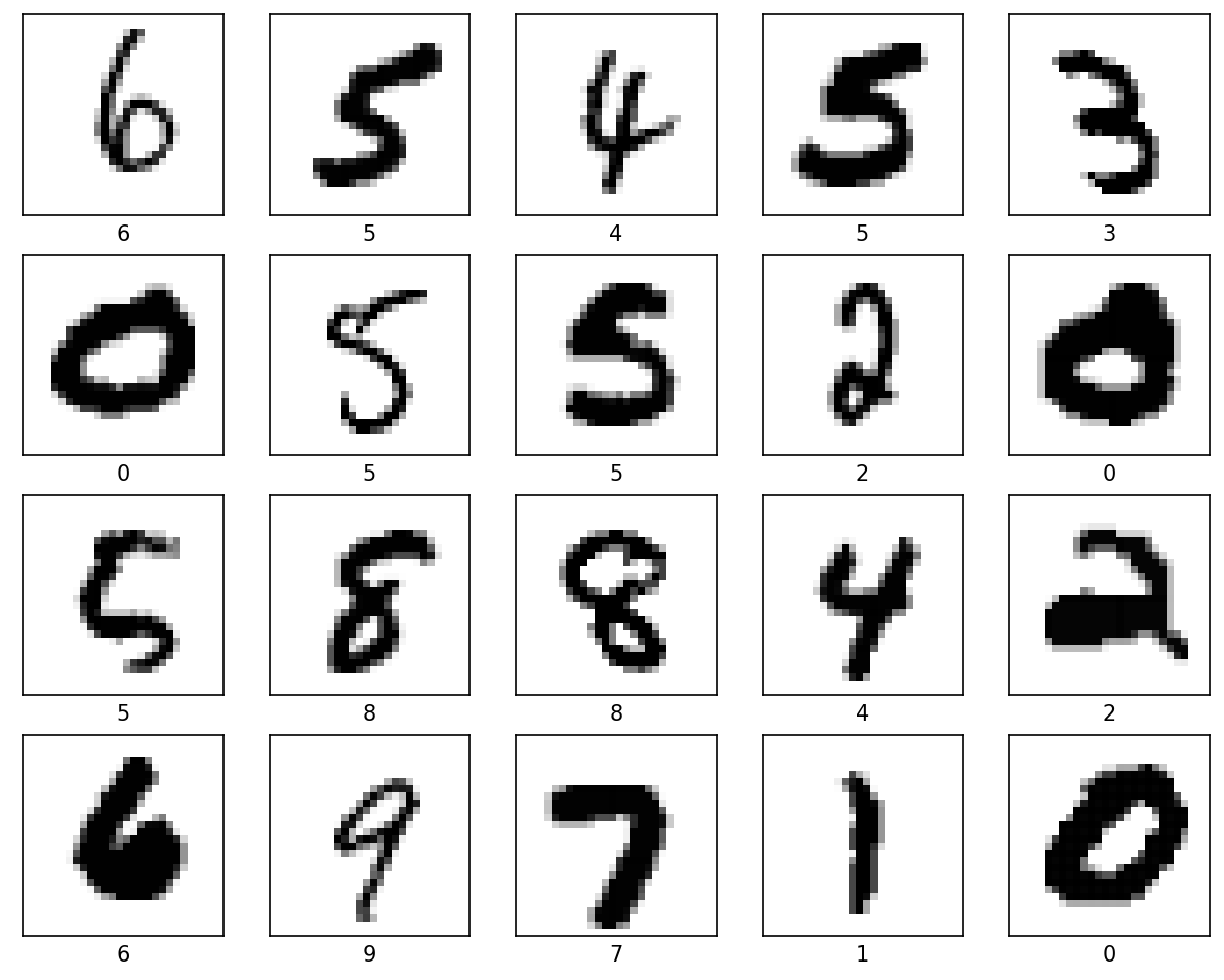
• 특성 데이터를 시각화 해보면 다음과 같은 숫자 손글씨임을 확인할 수 있다.

label_list = list(np.unique(y_test))

fig, ax = plt.subplots(figsize=(10,10))

for i, val in enumerate(range(attention_idx-10,attention_idx+10)):
    plt.subplot(5,5,i+1)
    plt.xticks([])
    plt.yticks([])
    plt.grid(False)
    plt.imshow(x_train[val], cmap=plt.cm.binary)
    plt.xlabel(label_list[y_train[val]])
plt.show()

데이터 전처리

x_train, x_test = x_train / 255, x_test / 255 # Normalization
x_train[attention_idx][10] # 2,000번 인덱스 살펴보기

• 데이터를 255로 나누어 0~1사이의 수로 정규화(Normalization)한다.
• 정규화 하는 이유?
  • 0~1 사이로 맞추어 계산 값이 너무 커지는 것을 방지
  • Local Minimun에 빠지는 것을 방지(학습 속도 향상)

모델링

인공신경망 구성

model = tf.keras.models.Sequential([
  Flatten(input_shape=(28, 28)),
  Dense(128, activation='relu'),
  Dropout(0.2),
  Dense(10, activation='softmax')
])

model.compile(optimizer='adam',
              loss='sparse_categorical_crossentropy',
              metrics=['accuracy'])

• 28픽셀이 흑백 이기 때문에 입력특성에는 (28, 28)로 입력한다.
• 은닉층의 노드는 128, 활성화 함수는 relu로 설정
• 과적합을 막기위하여 Dropout 0.2 설정
• 출력은 0~9까지의 숫자이기 때문에 10, 다중분류 함수인 softmax로 설정

신경망 학습

model.fit(x_train, y_train, epochs=5)

model.evaluate(x_test,  y_test, verbose=2)

313/313 - 0s - loss: 0.0724 - accuracy: 0.9775 - 488ms/epoch - 2ms/step
[0.0723787322640419, 0.9775000214576721]

• 5번 순전파와 역전파를 반복하며 신경망을 학습
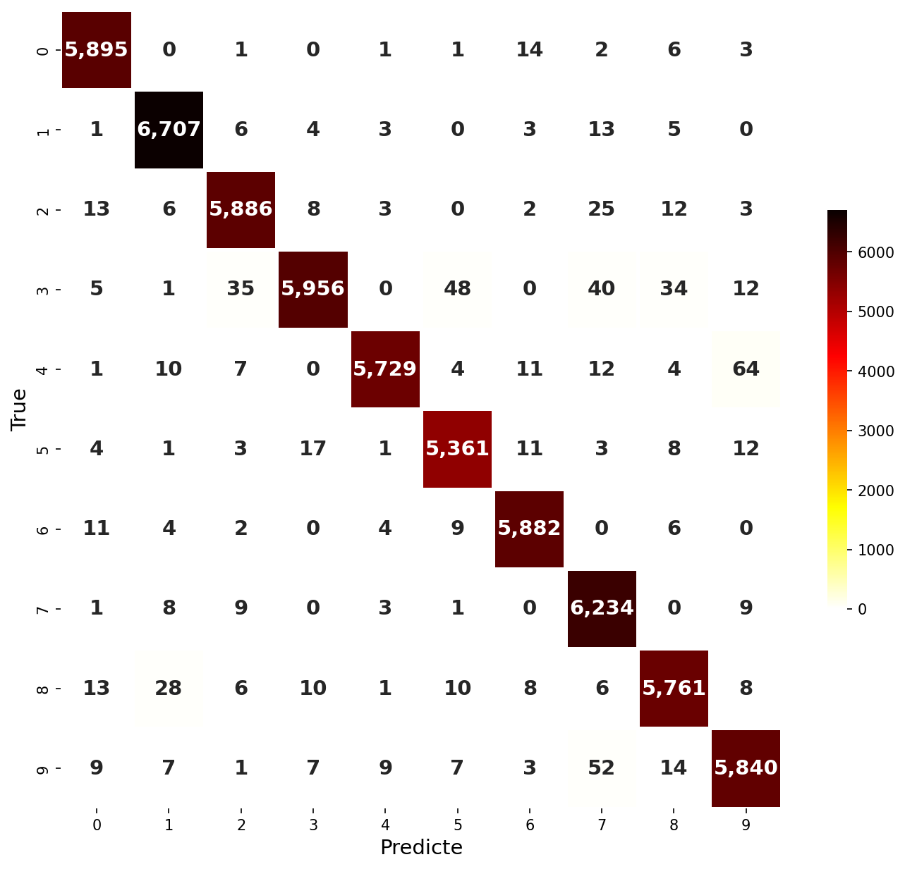
• 평가 데이터에 대하여 Accuracy를 반환
• 정확도 약 97.8%
• 혼돈행렬(Confusion Matrix)을 확인해보면 대부분 맞춘 것을 확인 할 수 있다.

모델 확인

probability_model = tf.keras.Sequential([
  model,
  tf.keras.layers.Softmax()
])

pred_list = probability_model(x_train[attention_idx:attention_idx+1])
predictions_train = probability_model.predict(x_train)
predictions_test = probability_model.predict(x_test)
pred_list

1875/1875 [==============================] - 2s 1ms/step
313/313 [==============================] - 0s 1ms/step
<tf.Tensor: shape=(1, 10), dtype=float32, numpy=
array([[0.09005527, 0.08849514, 0.08866849, 0.08850201, 0.08851673,
        0.1622487 , 0.12685911, 0.08853356, 0.08893044, 0.08919058]],
      dtype=float32)>

• 훈련데이터 2,000번 인덱스의 모델추정 결과 0,1,2,3,4일 확률은 약9%, 5일 확률은 약16%, 6일 확률은 약12.7%, 7,8,9일 확률은 약9%

np.argmax(predictions_train[attention_idx])
# 5

• 결국 모델의 선택은 5!!

• 훈련데이터 2,000번 인덱스를 확인해보면

plt.figure()
plt.imshow(x_train[attention_idx], cmap='gray_r')
plt.colorbar()
plt.grid(False)
plt.show()

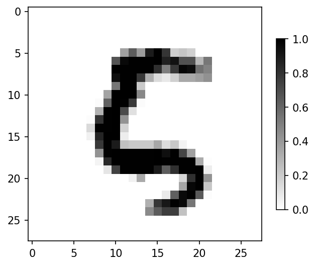
• 2,000번의 라벨을 확인해보면 5가 맞음

y_train[attention_idx]
# 5

끝까지 읽어주셔서 감사합니다😉