Fashion MNIST 인공신경망
Fashion MNIST, 인공신경망 구성
도입
- Fashion MNIST 데이터로 인공신경망 만들기
- 간단한 인공신경망을 구성하며 딥러닝과 친해지자
데이터 준비
데이터 읽어오기
# 데이터를 불러온다
(train_images, train_labels), (test_images, test_labels) = keras.datasets.fashion_mnist.load_data()
print(f"{train_images.shape},{train_labels.shape},{test_images.shape},{test_labels.shape}")
(60000, 28, 28),(60000,),(10000, 28, 28),(10000,)
- Fashion MNIST 데이터는 MNIST와 함께 딥러닝의 ‘Hellow, World!’와 같은 데이터이다.
- keras.datasets.fashion_mnist.load_data() 메써드는 넘파이 튜플을 반환한다.
- 학습데이터는 60,000개, 평가데이터는 10,000개이다.
- 28픽셀의 흑/백 특성을 담고 있다.
데이터 정규화
- 데이터를 255로 나누어 0~1사이의 수로 정규화(Normalization)한다.
- 정규화 하는 이유?
- 0~1 사이로 맞추어 계산 값이 너무 커지는 것을 방지
- Local Minimun에 빠지는 것을 방지(학습 속도 향상)
- 훈련데이터 인덱스20,000번 데이터의 정규화 하기 이전 값 살펴보기
train_images[attention_train][10]
array([  0,   0,   0,   0,   0,   0,   0,   0,   2,   0,   0,   0,   0,
       160, 255, 217, 255,  94,   0,   0,   0,   1,   4,   0,   0,   0,
        65,  38], dtype=uint8)
- 정규화 실행 $x - x_{min} \over x_{max} - x_{min}$
- 최소값이 0이기 때문에 최대값(255)로 나누기만 하였다
train_images = train_images / 255.0
test_images = test_images / 255.0
array([0.        , 0.        , 0.        , 0.        , 0.        ,
       0.        , 0.        , 0.        , 0.00784314, 0.        ,
       0.        , 0.        , 0.        , 0.62745098, 1.        ,
       0.85098039, 1.        , 0.36862745, 0.        , 0.        ,
       0.        , 0.00392157, 0.01568627, 0.        , 0.        ,
       0.        , 0.25490196, 0.14901961])
데이터 살펴보기
- 타겟 라벨 확인하기
class_names = ['T-shirt/top', 'Trouser', 'Pullover', 'Dress', 'Coat',
               'Sandal', 'Shirt', 'Sneaker', 'Bag', 'Ankle boot']
print(pd.DataFrame({'Label':class_names}).to_markdown())
| Label | |
|---|---|
| 0 | T-shirt/top |
| 1 | Trouser |
| 2 | Pullover |
| 3 | Dress |
| 4 | Coat |
| 5 | Sandal |
| 6 | Shirt |
| 7 | Sneaker |
| 8 | Bag |
| 9 | Ankle boot |
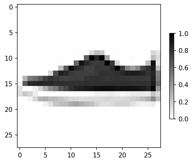
- 훈련데이터 인덱스20,000번 데이터를 시각화 해보자
plt.imshow(train_images[attention_train], cmap='gray_r')
plt.colorbar(shrink = .4)
plt.grid(False)
plt.show()
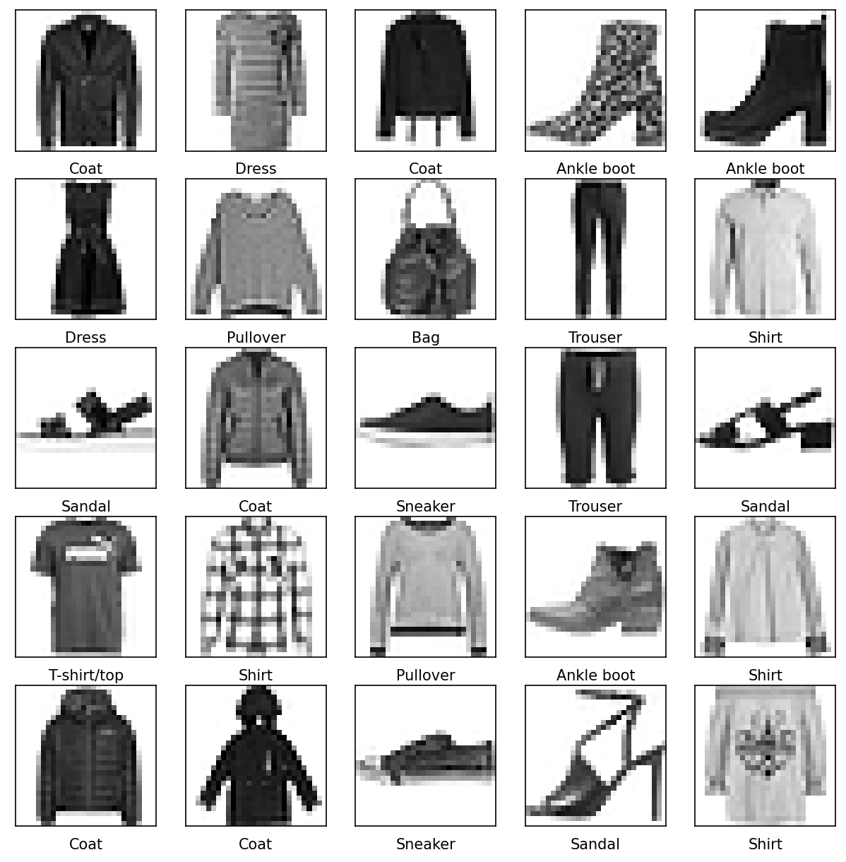
- 훈련데이터 25개 데이터를 시각화 해보자
for i, val in enumerate(range(attention_train-12,attention_train+13)):
    plt.subplot(5,5,i+1)
    plt.xticks([])
    plt.yticks([])
    plt.grid(False)
    plt.imshow(train_images[val], cmap=plt.cm.binary)
    plt.xlabel(class_names[train_labels[val]])
plt.show()
모델링
모델 구성하기
model = tf.keras.Sequential([
    tf.keras.layers.Flatten(input_shape=(28, 28)),
    tf.keras.layers.Dense(128, activation='relu'),
    tf.keras.layers.Dense(10, activation='softmax')
])

model.compile(optimizer='adam',
              loss=tf.keras.losses.SparseCategoricalCrossentropy(from_logits=True),
              metrics=['accuracy'])
- 28픽셀 흑백 데이터이기 때문에 입력층에는 (28, 28)로 입력한다.
- 은닉층의 노드는 128개, 활성화함수는 relu를 사용했다.
- 출력층은 10개 노드와 softmax 활성화함수를 지정하였다.
모델 학습하고 평가하기
model.fit(train_images, train_labels, epochs=10)
test_loss, test_acc = model.evaluate(test_images,  test_labels, verbose=2)
print('\nTest accuracy:', test_acc)
Epoch 1/10
1875/1875 [==============================] - 7s 3ms/step - loss: 0.4966 - accuracy: 0.8267
Epoch 2/10
1875/1875 [==============================] - 5s 3ms/step - loss: 0.3765 - accuracy: 0.8638
Epoch 3/10
1875/1875 [==============================] - 6s 3ms/step - loss: 0.3392 - accuracy: 0.8759
Epoch 4/10
1875/1875 [==============================] - 5s 3ms/step - loss: 0.3156 - accuracy: 0.8855
Epoch 5/10
1875/1875 [==============================] - 5s 3ms/step - loss: 0.2979 - accuracy: 0.8905
Epoch 6/10
1875/1875 [==============================] - 6s 3ms/step - loss: 0.2817 - accuracy: 0.8958
Epoch 7/10
1875/1875 [==============================] - 5s 3ms/step - loss: 0.2686 - accuracy: 0.9003
Epoch 8/10
1875/1875 [==============================] - 6s 3ms/step - loss: 0.2586 - accuracy: 0.9033
Epoch 9/10
1875/1875 [==============================] - 5s 3ms/step - loss: 0.2477 - accuracy: 0.9072
Epoch 10/10
1875/1875 [==============================] - 6s 3ms/step - loss: 0.2401 - accuracy: 0.9104
313/313 - 0s - loss: 0.3328 - accuracy: 0.8863 - 488ms/epoch - 2ms/step

Test accuracy: 0.8863000273704529
- 순전파와 역전파를 10번 반복하여 신경망을 학습한다.
- 평가데이터에 대하여 정확도를 산출
- 평가정확도 88.6%
모델 확인하기
- 모델 추정
probability_model = tf.keras.Sequential([model, keras.layers.Softmax()])
predictions = probability_model.predict(test_images)
평가 인덱스 2,000번, 모델 추정
- 모델은 8번(Bag)이라 예측
- 추정이 맞는지 확인해 보자
i = test_1
plt.figure(figsize=(6,3))
plt.subplot(1,2,1)
plot_image(i, predictions[i], test_labels, test_images)
plt.subplot(1,2,2)
plot_value_array(i, predictions[i],  test_labels)
plt.xticks(range(10), class_names, rotation=90)
plt.show()
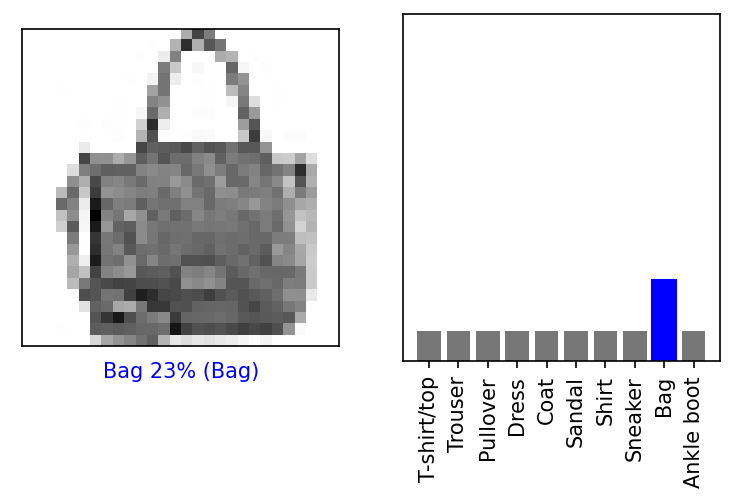
- 맞았다~!😄
평가 인덱스 800번, 모델 추정
- 모델은 9번(Ankle boot)이라 예측
- 추정이 맞는지 확인해 보자
i = test_2
plt.subplot(1,2,1)
plot_image(i, predictions[i], test_labels, test_images)
plt.subplot(1,2,2)
plot_value_array(i, predictions[i],  test_labels)
plt.xticks(range(10), class_names, rotation=90)
plt.show()
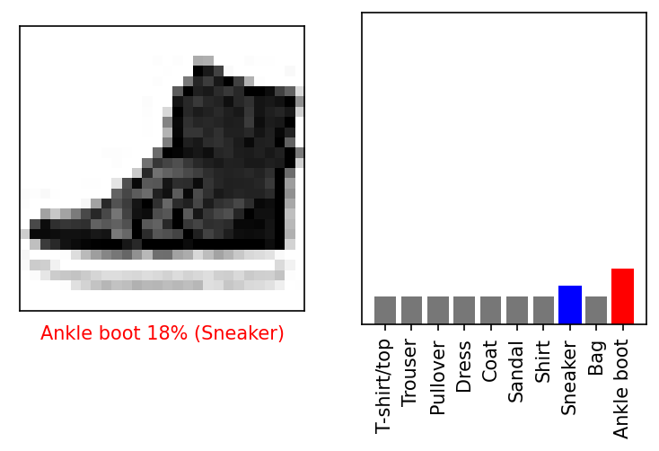
- 틀렸다…😥
평가데이터 15개 추정
num_rows = 5
num_cols = 3
num_images = num_rows*num_cols

fig, ax = plt.subplots( figsize=(2*2*num_cols, 2*num_rows) )

for i in range(num_images):
  plt.subplot(num_rows, 2*num_cols, 2*i+1)
  plot_image(i, predictions[i], test_labels, test_images)
  plt.subplot(num_rows, 2*num_cols, 2*i+2)
  plot_value_array(i, predictions[i], test_labels)
plt.tight_layout()
plt.show()
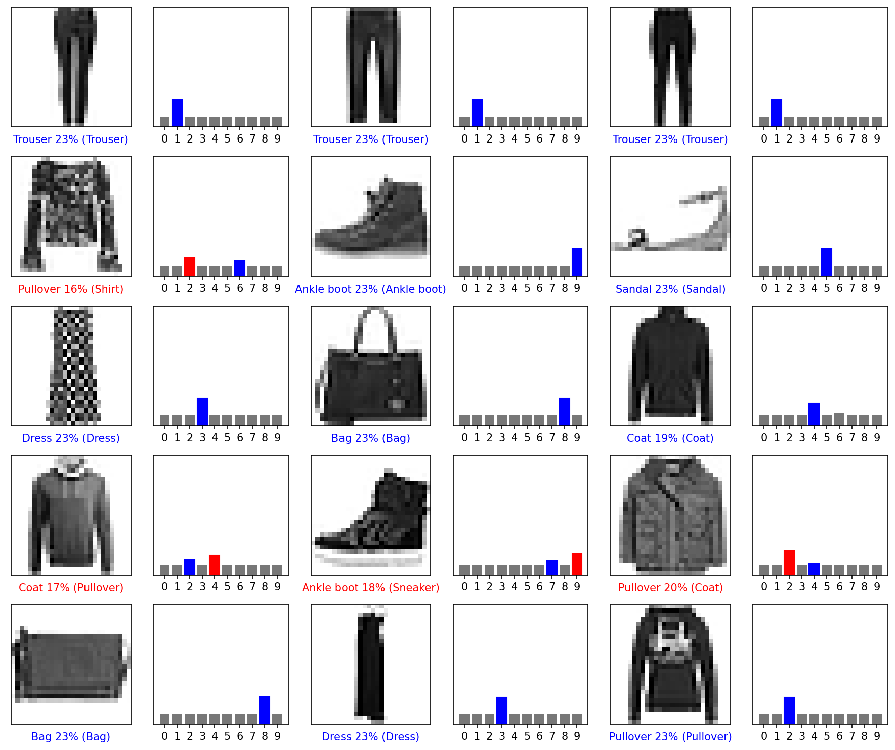
- 모델이 대부분 맞혔는데(파란색), 틀린것(빨간색)도 있다
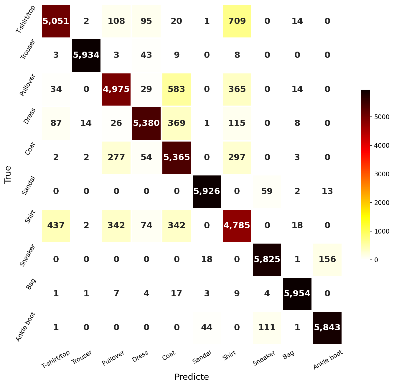
혼돈행렬(Confusion Matrix)
끝까지 읽어주셔서 감사합니다😉


댓글남기기